OFDM and the DFT

Shows how Orthogonal Frequency Division Multiplexing (OFDM) is implemented with a Discrete Fourier Transform (DFT), and how it relates to single carrier digital communications.
Related videos: (see: http://www.iaincollings.com)
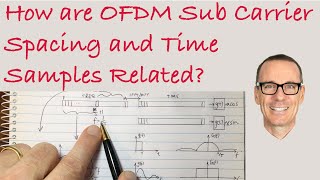
• How are OFDM Sub Carrier Spacing and Time Samples Related? https://youtu.be/knjeXo3VZvc
• Why is the OFDM Symbol Prefix Shorter in 5G Mobile and 802.11ac WiFi? https://youtu.be/a0aGVPkTOCI
• OFDM Waveforms: https://youtu.be/F6B4Kyj2rLw
• Why is Subcarrier Spacing Bigger in 5G Mobile Communications? https://youtu.be/uyDvjpPn8ms
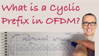
• What is a Cyclic Prefix in OFDM? https://youtu.be/AJg57AEBtNw
• How does OFDM Overcome ISI? https://youtu.be/xcQ6rtIXv6M
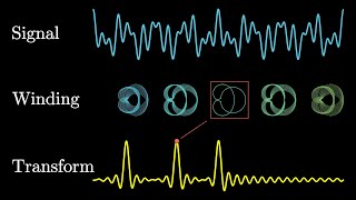
• Orthogonal Basis Functions in the Fourier Transform: https://youtu.be/n2kesLcPY7o
For a full list of Videos and Summary Sheets, goto: http://www.iaincollings.com

** Note: I gave the continuous-time version of the Inverse Fourier Transform equation because it's more intuitive to show how the waveforms (at the different frequencies) add up. But if you substitute t=(n/N)T, then you get the standard IDFT equation (in terms of the discrete-time samples, indexed by the variable n). This is because in the IDFT, there are N time-domain samples, which is because there are N frequency-domain subcarriers. I also didn't show the usual scaling by a factor of 1/N (which I probably should have mentioned. ... but it's just a scaling, so it doesn't change any of the intuition, which is what I am trying to show in the video).